How to Create Leave Tracker in Excel (With Easy Steps)

We’ll use a dataset of 5 employees of a company to create a leave tracker.

Step 1 – Create a Summary Layout

Create a Summary sheet.
Select cell F1.
From the Insert tab, select the drop-down arrow for Illustrations.
Choose Picture and select This Device.

A dialog box called Insert Picture will appear.
Select your company logo and click Insert.

We are inserting our website logo to show the process.

Select the range of cells B4:I4 and select the Merge & Center option from the Alignment group.
Insert the title. We set the file title as Employee Leave Tracker. Keep your desired formatting to the cell.

In the range of cells K8:L14, specify the leave types and their short codes. We put 6 different types of leaves.

Select cell B8:I8.
Select the Merge & Center option and write down the table title. We put it as Year Summary.

In cell B9, write the column name as Employee Name and set the range of cells B10:B14 for 5 employees.

In the range of cells C9:H9, denote the leave short forms.

Set 2 Total cells, one for the column and the other for the rows.

Here’s our summary layout.

Step 2 – Build Tracker List for Each Month

Create a new sheet and rename it as Jan.
In the Home tab, select the Format option from the Cells group and click on Column Width.

A small dialog box called Column Width will appear.
Set the column width to 2.50 and click OK.

Select cell AF1 and insert your company logo similarly as in Step 1.

In cell B4, insert the following formula:

="January"&Summary!C6

Press Enter to store the data.

As the month of January has 31 days, select 32 columns that are from B6:AG6. Select the Merge & Center option from the Alignment group.
In the merged cell, insert the following formula and press the Enter key.

=B4

Modify the cell format for the range of cells B9:B13 and keep them to input the employee names.

=DATE(Summary!$C$6,1,1)

In cell D8, insert the following formula and drag the Fill Handle icon to the right to copy the formula until you get 28.

=C8+1

For the last 3 cells AE8:AG8, insert the formula shown below:

=IF(MONTH($AD8+1)>MONTH($C$8),"",$AD8+1)

Breakdown of the Formula

MONTH($AD8+1): This function returns 1.

MONTH($C$8): This function returns 1.

IF(MONTH($AD8+1)>MONTH($C$8),””,$AD8+1): This function returns the date.

In cell C7, insert the following formula:

=IF(C8="","",INDEX(,WEEKDAY(C8,1)))

Breakdown of the Formula

WEEKDAY(C8,1): This function returns 7.

INDEX(,WEEKDAY(C8,1)): This function returns Sa.

IF(C8=””,””,INDEX(,WEEKDAY(C8,1))): This function returns the day name Sa.

Drag the Fill Handle icon to the right to copy the formula up to cell AG7.

Select cell C9.
In the Data tab, select the drop-down arrow of the Data Validation option from the Data Tools group.
Select the Data Validation option.

A small dialog box called Data Validation will appear.
In the Setting tab, select the drop-down arrow below the Allow title and choose the List option.
Insert the cell reference $AH$8:$AM$8 in the box below Source or simply select the range with your mouse.
Click OK.

You will see a drop-down arrow that contains all the short forms.
Drag the Fill Handle icon in the range of cells C9:AG13 to copy the drop-down arrow in all the cells.
Mark the weekends with a different color so that you can easily find them.

Select the range of cells AH6:AM6 and choose the Merge & Center option.
Name the merged cell as Total.

Use the COUNTIF function in the following formula in cell AH9:

=COUNTIF($C9:$AG9,AH$8)+0.5*COUNTIF($C9:$AG9,AH$8&"H")+0.5*COUNTIF($C9:$AG9,"H"&AH$8)

Breakdown of the Formula

COUNTIF($C9:$AG9,AH$8): This function returns 1.

COUNTIF($C9:$AG9,AH$8&”H”): This function returns 0.

COUNTIF($C9:$AG9,”H”&AH$8): This function returns 0.

COUNTIF($C9:$AG9,AH$8)+0.5*COUNTIF($C9:$AG9,AH$8&”H”)+0.5*COUNTIF($C9:$AG9, “H”&AH$8): This function returns the day name 1.

Drag the Fill Handle icon to the range of cells AH9:AM13.

In the range of cells AH8:AM8, insert the following formula to show the leave type short forms.

=Summary!C9

=SUM(AH9:AH13)

Drag the Fill Handle icon to copy the formula up to cell AM7.
The leave tracker for the month of January will be ready to use.

Create the monthly leave tracker sheets for the other months of the year. You can copy most of the content and change the month.

Step 3 – Generate the Final Leave Tracker

Insert the following formula into cell C9.

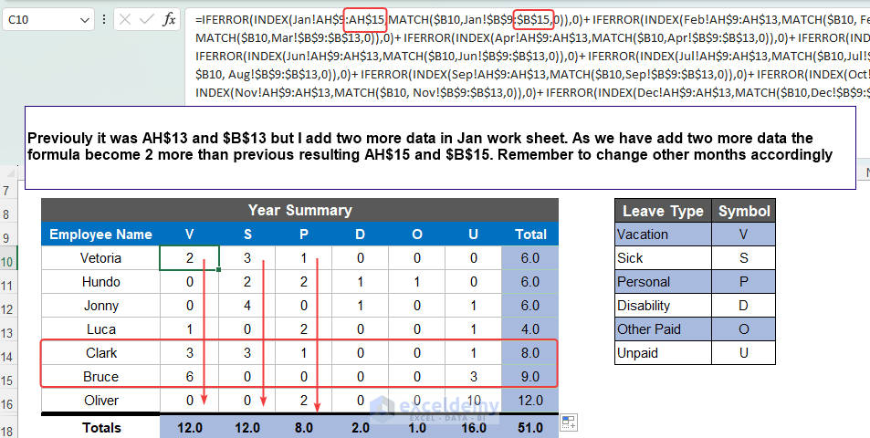
=IFERROR(INDEX(Jan!AH$9:AH$13,MATCH($B10,Jan!$B$9:$B$13,0)),0)+IFERROR(INDEX(Feb!AH$9:AH$13,MATCH($B10,Feb!$B$9:$B$13,0)),0)+IFERROR(INDEX(Mar!AH$9:AH$13,MATCH($B10,Mar!$B$9:$B$13,0)),0)+IFERROR(INDEX(Apr!AH$9:AH$13,MATCH($B10,Apr!$B$9:$B$13,0)),0)+IFERROR(INDEX(May!AH$9:AH$13,MATCH($B10,May!$B$9:$B$13,0)),0)+IFERROR(INDEX(Jun!AH$9:AH$13,MATCH($B10,Jun!$B$9:$B$13,0)),0)+IFERROR(INDEX(Jul!AH$9:AH$13,MATCH($B10,Jul!$B$9:$B$13,0)),0)+IFERROR(INDEX(Aug!AH$9:AH$13,MATCH($B10,Aug!$B$9:$B$13,0)),0)+IFERROR(INDEX(Sep!AH$9:AH$13,MATCH($B10,Sep!$B$9:$B$13,0)),0)+IFERROR(INDEX(Oct!AH$9:AH$13,MATCH($B10,Oct!$B$9:$B$13,0)),0)+IFERROR(INDEX(Nov!AH$9:AH$13,MATCH($B10,Nov!$B$9:$B$13,0)),0)+IFERROR(INDEX(Dec!AH$9:AH$13,MATCH($B10,Dec!$B$9:$B$13,0)),0)

Breakdown of the Formula

MATCH($B10,Jan!$B$9:$B$13,0): This function returns 2.

INDEX(Jan!AH$9:AH$13,MATCH($B10,Jan!$B$9:$B$13,0)): This function returns 0.

IFERROR(INDEX(Jan!AH$9:AH$13,MATCH($B10,Jan!$B$9:$B$13,0)),0): This function returns 1.

Copy the formula up to cell H14 by dragging the Fill Handle icon.

In cell I10, use the SUM function to sum the range of cells C10:H10:

=SUM(C10:H10)

Double-click on the Fill Handle icon to copy the formula up to cell I14.

In cell C16, insert the following formula:

=SUM(C10:C14)

Copy the formula up to cell I16 using the Fill Handle icon.

The leave tracker is completed and ready to use.

Step 4 – Verify the Leave Tracker with Data

Input employee names in the range of cells B10:B14.
Input some data for January in the sheet Jan.

Input some values for the months of February in sheets Feb.

If you check the Year Summary table, you will find our formula is extracting the values from the month sheets and showing us individual employees and individual leave types.

Save Saved Removed 0 Soumik Dutta

Soumik Dutta, having earned a BSc in Naval Architecture & Engineering from Bangladesh University of Engineering and Technology, plays a key role as an Excel & VBA Content Developer at ExcelDemy. Driven by a profound passion for research and innovation, he actively immerses himself in Excel. In his role, Soumik not only skillfully addresses complex challenges but also demonstrates enthusiasm and expertise in gracefully navigating tough situations, underscoring his unwavering commitment to consistently deliver exceptional, high-quality content that. Read Full Bio

15 Comments

Hi! Am Babalola Olona. I want to say a very big thank you to ExcelDemy for this great article as this will go a long way to help build up a lot of learners. While I am happy that am able to learn a lot from this piece I however have challenges comprehending Step 3 “Generate Final Leave Tracker”, I really cant understand the formula used “IFERROR, INDEX, MATCH & SUM”. I can’t also understand the rational behind the use of 0.5, “H” & in the COUNTIF function. i will be eternally grateful this FUNCTIONS can be further broken down for a better understanding. Thank you.

Naimul Hasan Arif Apr 5, 2023 at 12:02 PM

Thanks a lot BABALOLA for the appreciation. It means a lot.
In response to your first question, let me break down the whole formula with IFERROR, INDEX, MATCH & SUM and explain it to you. The first part of the formula here is IFERROR(INDEX(Jan!AH$9:AH$13,MATCH($B10,Jan!$B$9:$B$13,0)),0)
First of all the MATCH function looks through the value in range B9:B13 of Jan sheet whether it matches the value in cell B10. If it gets matched, it will return the related value according to the index from the AH9:AH13 range. The IFERROR Function is used to return a value(i.e. 0) if it can not find any proper value to return.
Similarly, I have gone through all 12 months’ sheets and added them with the SUM function. In response to your second question, the & sign is used to concatenate cell AH$8 with the letter H. As it is considered a half match, 0.5 is multiplied. We have considered two half-matches to have the full match count.

Karlyn Martinez Aug 2, 2023 at 3:19 AM

Hello, I track leave for my company and need more rows than 5 (much more than 5 people), how do I insert rows without messing up the formula?

Joyanta Mitra Aug 2, 2023 at 1:11 PM

Dear Karlyn Martinez,
For your convenience, I have showed the task with following steps.
Steps:
● First, you have to recognize the pattern in the formula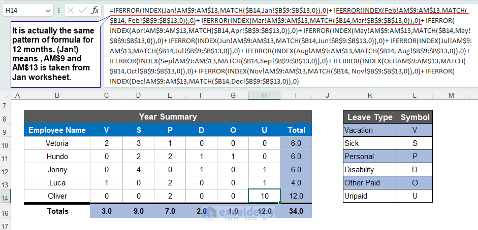
Showing pattern
● You can use Format Painter or drag the row to add a new row or rows for editing new data. 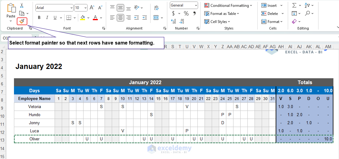Modifying data
● Now add new data. 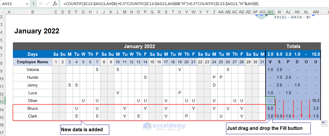Adding new data
● Inset new rows in the Summary sheet.
Inserting new rows in Summary sheet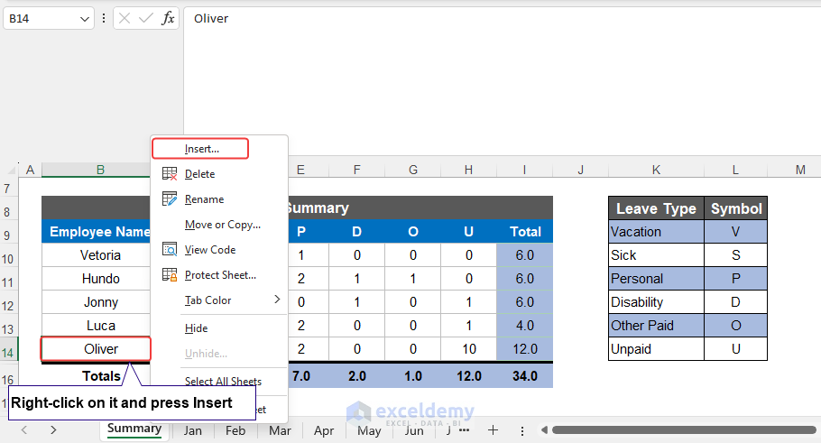
● Insert the Entire row.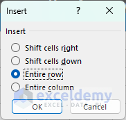

● Edit the code according to the main dataset. As now in Jan worksheet, new data is added, and so the range will be changed to AH$15 and $B$15.
Showing the formula change Hope, this will be helpful for you. Regards,
Joyanta Mitra
Excel & VBA Content Developer

We ran into issues with the large formula since our line number weren’t exactly like yours. For instance, I have 10 employees vs 7. We’re still working on it but not quite there yet. Wish there was an easier way to get the summary.

How do you record half day leave?

Aniruddah Alam Jan 15, 2024 at 9:39 AM

Hi KOH, Thanks for reaching out to us! Unfortunately, the method discussed above doesn’t currently support recording half-day leave. We understand how frustrating that can be, and we’re sorry for any inconvenience caused. Rest assured, we’ll definitely work on overcoming this limitation in the future. We’re grateful for your support of Exceldemy and we hope to make your experience even better in the future. Best regards,
Aniruddah
Team Exceldemy

Hello – this tutorial has been so helpful – THANK YOU! I am however struggling to get my summary to pick up leave noted throughout the year when i carry out my test (as you do in your video)……I cannot work out where I have made an error as I thought I was being very careful to follow all of your instructions….can you please provide any help?

Lutfor Rahman Shimanto Mar 24, 2024 at 4:28 PM

Hello Tracey Thanks for your nice words. Your appreciation means a lot to us. Creating a Leave Tracker in Excel requires multiple steps, so you may often get unintentional errors when following these steps. Do not worry! You can share your problem within the ExcelDemy Forum by attaching your workbook. Regards
ExcelDemy

Hello
I am not having any luck with step 3 generate final leave tracker on the summary page. I have tried it many different ways with no luck. Can I send it to get some help?

Lutfor Rahman Shimanto Mar 27, 2024 at 5:09 PM

Hello Bonnie Thanks for reaching out. Though a few steps are needed, making mistakes along the way is obvious. But no worries! The ExcelDemy Forum is there to help. Just share your workbook and ask for advice. Regards
Lutfor Rahman Shimanto
ExcelDemy

I have 100 employees. I made it but the summary doesn’t work!!

Lutfor Rahman Shimanto May 19, 2024 at 12:20 PM

Dear Sanjeev Thanks for visiting our blog and sharing your problem. After adding the desired rows, you must drag the Fill Handle icon to copy the existing formulas for new employees. We have improved the file and made the necessary formula adjustments based on your goal. SOLUTION Overview: You can download the solution file: https://www.exceldemy.com/wp-content/uploads/2024/05/Sanjeev-Fernandes-SOLVED.xlsx Regards
Lutfor Rahman Shimanto
ExcelDemy

Great work guys. Your patience and responses

Shamima Sultana Aug 17, 2024 at 11:31 AM

Hello Babajide, Thanks! We are glad to hear that you found it great. We try our best to provide excellent services. Keep learning Excel with ExcelDemy! Regards
ExcelDemy