
We propose an approach for learning optimal tree-based prescription policies directly from data, combining methods for counterfactual estimation from the causal inference literature with recent advances in training globally-optimal decision trees. The resulting method, Optimal Policy Trees, yields interpretable prescription policies, is highly scalable, and handles both discrete and continuous treatments. We conduct extensive experiments on both synthetic and real-world datasets and demonstrate that these trees offer best-in-class performance across a wide variety of problems.
Avoid common mistakes on your manuscript.
The ever-increasing availability of high-quality and granular data is driving a shift away from one-size-fits-all policies towards personalized and data-driven decision making. In medicine, different treatment courses can be recommended based on individual patient characteristics rather than following general rules of thumb. In insurance, underwriting decisions could be made at the individual level, rather than relying on aggregate populations and actuarial tables. In e-commerce, consumers may experience a personalized version of a website, tailored to their shopping tastes. In all domains, the ability to understand the underlying phenomena in the data to aid decision making is critical.
In this paper, we consider the problem of determining the best prescription policy for assigning treatments to a given observation (e.g. a customer or a patient) as a function of the observation’s features. A common context is that we have observational data of the form \(\left\< (\varvec<\mathbf
Decision trees are an appealing class of model to apply to this problem, as their interpretability and transparency allows humans to inspect and understand the decision-making process, to both develop their understanding of the underlying phenomenon and to identify and correct flaws in the model. The interpretability is arguably more important in prescriptive problems than in predictive problems, as a prescriptive model recommends actions with direct and often significant consequences, requiring more transparency and justification than models that simply make predictions.
One of the key difficulties in learning from observational data is the lack of complete information. In the data, we only observe the outcome corresponding to the treatment that was applied. Crucially, we do not observe what would have happened if we had applied other treatments to each observation, the so-called counterfactual outcomes.
Previous approaches (Bertsimas et al. 2019; Kallus 2017) for decision tree-based prescriptions from observational data dealt with the lack of information by embedding a counterfactual estimation model inside the prescriptive decision tree, combining the tasks of estimating the counterfactuals and learning the optimal prescription policy. While this approach has the attractive property of learning from the data in a single step, it also makes the learning problem more complicated and thus limits the complexity of counterfactual estimation to approaches than can be practically embedded in a tree-training process.
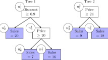
Some recent works (Biggs et al. 2020; Zhou et al. 2018) have proposed decision tree approaches to this problem that separate the counterfactual estimation and policy learning steps. Instead of a single learning step, the counterfactuals are first estimated using a method that models the data well, and than a decision tree is trained against these estimates to learn an optimal prescription policy (see Table 1 for an example of the counterfactual estimation process). These approaches use greedy heuristics to train the decision trees, rather than aiming for global optimality (Zhou et al. 2018 also include an exhaustive tree search, which does not scale beyond shallow trees and small datasets).
While the tree looks similar to a classification tree, there is an important difference in how they are trained. A classification tree focuses only on whether the predicted label is correct, whereas the policy tree uses the rewards to take into account the relative cost of each treatment option. For instance, consider a setting with three treatment options and an observation with rewards under these treatments of [1, 2, 10]. Assuming that we seek to minimize the rewards, a classification view of this problem would deem that the first treatment (with the lowest reward) is the “correct” label, and we would get equal penalty for prescribing the second or third treatments. In contrast, the policy view of the problem would incur a relative penalty of 1 and 9 for prescribing the second and third treatments, respectively. In this way, the policy tree makes use of the relative values of the rewards rather than simply focusing on which treatment gives the best reward for each observation.
We denote the leaf of the tree into which an observation \(\varvec<\mathbf
Combining (1) and (2) yields the following optimization problem:
$$\beginSpecifically, for each observation i, we identify the leaf \(\ell = v(\varvec<\mathbf
To solve Problem (3), we note that it is separable in the leaves of the problem:
$$\beginThis means that given a tree structure \(v(\varvec<\mathbf
which can be solved simply by enumerating the possible prescription options.
Note that this problem formulation is equivalent to the classification tree problem under misclassification loss, with the addition of per-observation, per-class losses \(\Gamma _\) . We can thus use any approach for training classification trees to solve this problem, provided that they support the specification of such custom loss weights.
In this case, we will utilize the Optimal Trees framework (Bertsimas and Dunn 2019) to optimize the tree structure and determine \(v(\varvec<\mathbf
where \(\text (v)\) is the number of splits in the tree v, and \(\text (v)\) is the depth of the tree. There are three hyperparameters that control the size of the resulting trees to prevent overfitting, and must be specified by the user:
The first two of these are the most critical parameters to tune, and the Optimal Trees framework details a tailored tuning algorithm for determining these parameters in Section 8.4 of (Bertsimas and Dunn 2019). For example, \(D_<\max >\) is tuned using a normal grid search over discrete values, whereas \(\alpha\) is tuned using a pruning procedure based on generating a sequence of related trees and finding the value of \(\alpha\) that would minimize the validation error.
As noted earlier, Problem (3) is also solved in the same fashion with a tree-based model by Biggs et al. (2020) and Zhou et al. (2018), but in both cases a greedy heuristic is used to train the tree. For other problem classes like classification and regression, there are significant performance and interpretability advantages to training trees with globally optimal methods rather than greedily (Bertsimas and Dunn 2017, 2019; Bertsimas et al. 2019). Our experiments in Sects. 4 and 5.1 demonstrate that this is also the case for the optimal policy problem.
In Sect. 3.1, we assumed that we had access to reward information \(\Gamma _\) for every observation i and every treatment option t. In some cases, we have access to this full information about the problem (see Sect. 5.3 for an example), but often we have observational data and thus only observe the outcome for the treatment that was applied in the data. In these cases, we will need to estimate the missing counterfactual outcomes. The method we use to estimate depends on the type of prescription decision being made.
When the prescription is a choice of one treatment from a set of possible options, we draw on the causal inference literature and use doubly-robust estimates (Dudík et al. 2011) for the outcomes, as outlined by Zhou et al. (2018) and Athey and Wager (2017).
For clarity, we present the estimation process here. There are three steps:
>_\) that a given observation i is assigned a given treatment t. We use the features \(\varvec<\mathbf
>_\) and outcomes \(<\hat
Using these estimated values \(\Gamma _\) in Eq. (1) results in a so-called doubly-robust estimate of the policy quality. This means that the estimated total reward under the policy has low bias if at least one of the propensity score or outcome sub-estimators has low bias, thus the name doubly-robust (Dudík et al. 2011).
Compared to using the outcome estimates directly as the rewards, an important advantage of the doubly-robust estimator is the ability to correct for treatment assignment bias in the observed data. Treatments in observational data are often not assigned at random, and this bias can influence the outcome estimation process, leading to poor estimates if not accounted for. For instance, consider a medical example where a specific treatment is typically given to sicker patients. This means that the group receiving this treatment is composed of sicker patients to begin with, and thus despite receiving the treatment, we might see that the outcomes in the treated group are lower than in the untreated group. This could cause the outcome estimator to predict lower outcomes when the treatment is applied, whereas in reality the treatment might still be helpful, as the outcomes in the treated group would be even worse without the treatment application. Combining the propensity scores with the outcome estimates helps to correct for any such treatment assignment bias in the data, to ensure that the estimated rewards are fair.
When the prescription is choosing the dosing level for one or more treatments, we estimate the counterfactual outcomes with a regression model.
We denote by \(z_\) the dose of each treatment t for each observation i, and treat the dose for each treatment as a separate continuous feature in the dataset. We then train a regression model (such as random forests or boosting) to predict the outcome \(y_i\) based on the features \(\varvec<\mathbf
Note that if the outcomes \(y_i\) are binary (e.g. denoting a success or failure), then a classification model can be used for estimation in place of regression. In this case, the estimated probabilities from the classification model can be used as the estimated outcomes.
To train and evaluate Optimal Policy Trees from observational data, we combine the approaches in Sects. 3.1 and 3.2. The exact workflow is:
To select the class of model and their associated hyperparameters for the reward estimation procedures in Steps 2 and 5, we recommend considering a range of model classes (e.g. boosted decision trees, random forests, linear regression) and using cross-validation to tune hyperparameters for each such model, before selecting the model class with the best estimated out-of-sample performance, so as to lead to high-quality reward estimates. Empirically, we have found that the highest estimated out-of-sample performance generally comes from boosted decision trees or random forests.
Note that in Step 5, training a separate estimation model in the test data purely serves the purpose of obtaining an unbiased evaluation of the policies, which is not necessary if the purpose is only for inference. In online settings where new observations arrive one-by-one, the Optimal Policy Tree model can still make prescriptions for these new observations, but we may not be able to provide a fair estimate of the policy performance for this new data.
Throughout this section, we have assumed that the reward \(\Gamma _\) for a given observation can depend on the features \(\varvec<\mathbf
In this section, we conduct a number of experiments on synthetically-generated data in order to evaluate the relative performance of optimal policy trees against other methods for prescriptive decision making.
Our experimental setup follows that used in Powers et al. (2018) and Bertsimas et al. (2019). We generate n data points \(\varvec<\mathbf
First, we consider scenarios with a single binary treatment. We define a baseline function that generates the baseline outcome for each observation, and an effect function that models the effect of the treatment being applied. The different functional forms we consider are presented in Table 2. Each function is further centered and scaled so that the generated values have zero mean and unit variance. In each experiment, we model the outcomes under “no treatment” and “treatment” ( \(Y_0\) and \(Y_1\) , respectively) as
We will adopt the convention that lower outcomes are desirable for all experiments. We assign treatments in a biased way to simulate an observational study where observations are more likely to receive the treatment option with the better outcome. Concretely, we assign the treatment with probability
The outcomes in the training set have additional i.i.d. noise added in the form \(\epsilon _i \sim \text (0, 0.1)\) .
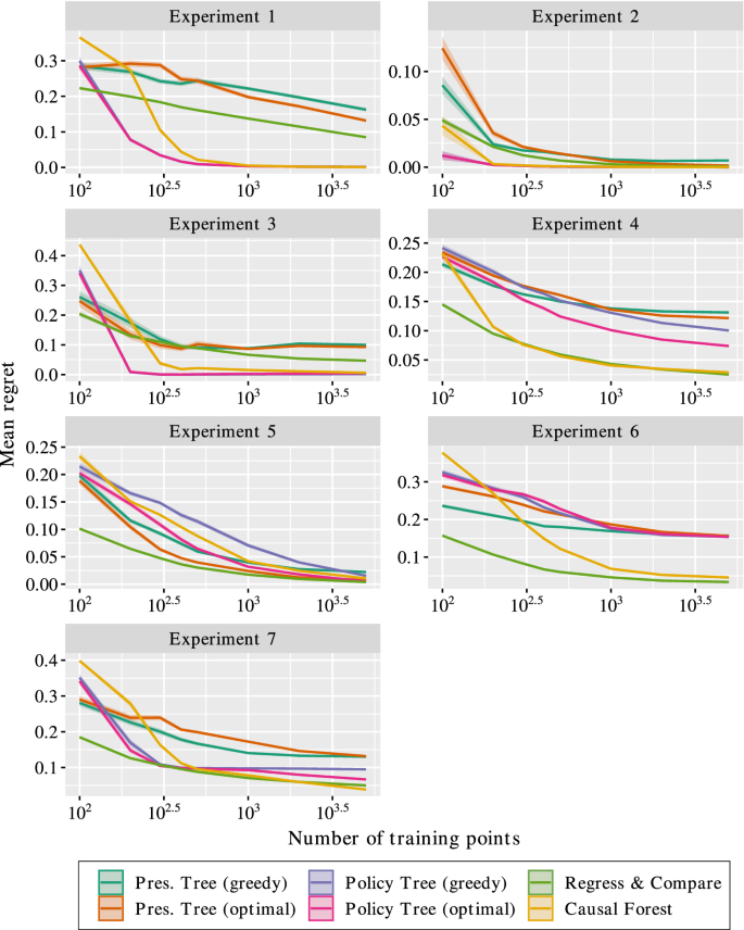
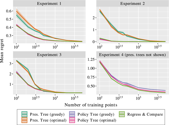
Figure 2 presents the results of the experiments. We make the following observations:
To summarize the results, the performance of policy trees depends on the nature of the effect function, but is largely independent of the baseline function. This is because the policy tree only considers the relative effects of each treatment and does not need to estimate the raw outcome under each treatment, and therefore does not depend on the complexity of the underlying baseline function. When the effect function can be modeled well by a tree structure, the policy trees pe rform among the best methods, with the optimal approach outperforming the greedy method when the solution is non-trivial. On the other hand, the performance of prescriptive trees depends heavily on the complexity of both baseline and effect functions, and perform worse than policy trees when the baseline is non-trivial. R&C and causal forests perform well in most cases, but suffer from a lack of interpretability and in some cases exhibit slower convergence than policy trees.
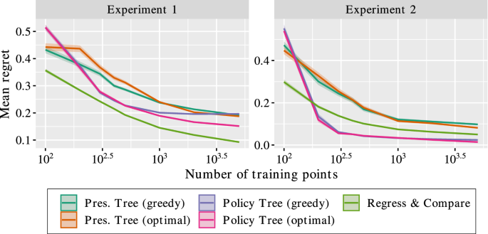
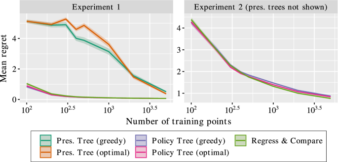
In this section, we extend the previous experiment setup to consider problems with more than two treatment options. We again borrow the setup from Bertsimas et al. (2019) and add an additional experiment. In this case, the outcomes are generated as
The treatments are assigned so that the “no treatment” option is more likely to be assigned when the baseline is small, and treatments 1 and 2 are equally likely to be assigned:
The experiments we consider as shown in Table 4. As before, the outcomes in the training set have additional i.i.d. noise added in the form \(\epsilon _i \sim \text (0, 0.1)\) . We again report the mean regret for each method on the testing set. Because there are multiple treatments, we do not include causal forests.
Now, we consider experiments where the outcomes are a continuous function of the treatment. In this case, our prescription is the dose level of the treatment to apply, rather than choosing one treatment option from the available set.
For these experiments, we define an outcome function \(y(\varvec<\mathbf
Our final set of experiments consider cases with multiple continuous-dose treatments. For these experiments, we define an outcome function \(y(\varvec<\mathbf
In addition to the relative performance of each method, we are also interested in comparing their runtimes. Table 8 shows the mean runtime in seconds for each method on each of the synthetic experiments discussed earlier. These reported runtimes are for the largest instance of each problem with \(n=5,000\) training points, and measure the complete time to run each method, including training, validation, and reward estimation for the policy tree methods.
In this section, we apply our algorithms to personalized diabetes management using patient-level data from Boston Medical Center, under a multi-treatment continuous dosing setup. This dataset was first considered by Bertsimas et al. (2017), where the authors propose a k-nearest neighbors (kNN) regress-and-compare approach, and was revisited by Bertsimas et al. (2019) with Optimal Prescriptive Trees.
This dataset consists of electronic medical records for more than 1.1 million patients from 1999 to 2014. We consider more than 100,000 patient visits for patients with type 2 diabetes during this period. The features of each visit include demographic information (sex, race, gender etc.), treatment history, and diabetes progression. The goal is to recommend a treatment regimen for each patient, where a regimen is a combination of oral, insulin, and metformin drugs and their dosages.
In the previous studies, the regress-and-compare and Optimal Prescriptive Trees approaches were limited to considering discrete treatments, so the treatment options were discretized into 13 different combinations, from which the method had to prescribe one choice to the patient. This has the unfortunate side effect of removing information about the proximity of different drug combinations. For instance, the combinations “insulin + metformin” and “insulin + metformin + 1 oral” are similar prescriptions, and it is plausible we may be able to learn shared information from patients that received either of these. On the other hand, “insulin” and “metformin + 2 oral” are very unrelated and we should not expect to use the patients receiving one of these to learn about the other.
When the treatments are discretized, all treatments are completely disjoint, and the rewards are learned separately, with no ability for shared learning where appropriate. Another approach is to view this problem as multiple continuous dose treatments. In this way, the treatment decision becomes the doses of insulin, metformin and oral drugs to apply, which we can view as a vector \((z_\mathrm , z_\mathrm , z_\mathrm )\) . From this perspective, the combinations “insulin + metformin”, (1, 1, 0), and “insulin + metformin + 1 oral”, (1, 1, 1), are indeed closer than “insulin”, (1, 0, 0) and “metformin + 2 oral”, (0, 1, 2), and thus we might expect that viewing the problem in this way could lead to more efficient learning due to the ability to share information across treatments.
We consider applying Optimal Policy Trees to this problem, both with 13 discrete treatment options and also with the continuous dosing model described earlier, to examine whether this more accurate model of the treatments indeed leads to better data efficiency. We used boosting to estimate the rewards in both the discrete and continuous-dose treatment models. To ensure fairness, the continuous-dose Optimal Policy Trees were required to prescribe from the same 13 treatment options, so any difference comes from better estimation due to a more accurate model of reality.
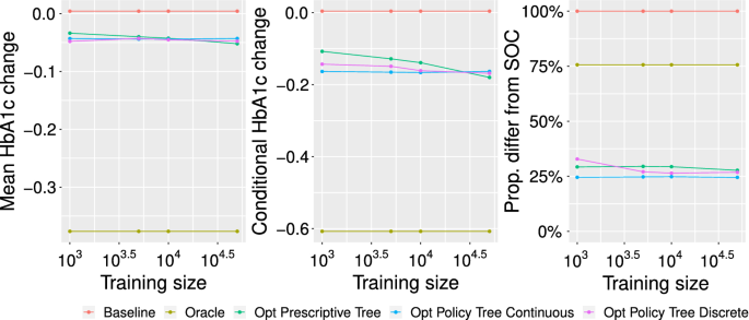
We follow the same experimental design as in Bertsimas et al. (2017). The quality of the predictions on the testing data is evaluated using a random-forest approach to impute the counterfactuals on the test set. We use the same three metrics to evaluate the various methods: the mean HbA1c improvement relative to the standard of care; the percentage of visits for which the algorithm’s recommendations differed from the observed standard of care; and the mean HbA1c benefit relative to standard of care for patients where the algorithm’s recommendation differed from the observed care. These metrics were selected because the reduction in HbA1c is considered clinically relevant.
We varied the number of training samples between 1,000 and 50,000 (with the test set fixed) to examine the effect of the amount of training data on out-of-sample performance. In addition to both Optimal Prescriptive Trees and Optimal Policy Trees (with both discrete and continuous treatment models), we consider the performance of a baseline method that continues the current line of care, and an oracle method that prescribes the best treatment for each patient is selected according to the estimated counterfactuals on the test set.
In Fig. 7, we show the performance across these methods. We observe that while all three tree methods converge to roughly the same performance as all the data is used, the Optimal Policy Trees achieve much better results when the training set is smaller. In addition, the Optimal Policy Trees based on the continuous-dose reward model outperform those based on the discrete treatment reward model. In fact, we see that the performance of the continuous-dose policy trees is roughly constant regardless of the size of the training set, indicating it is extremely efficient with the data, and only requires 1,000 samples to deliver performance equivalent to the Optimal Prescriptive Trees with 50,000 samples. This is very strong evidence that separating the counterfactual estimation and policy learning steps and permitting shared learning across treatments enable extremely efficient use of data.
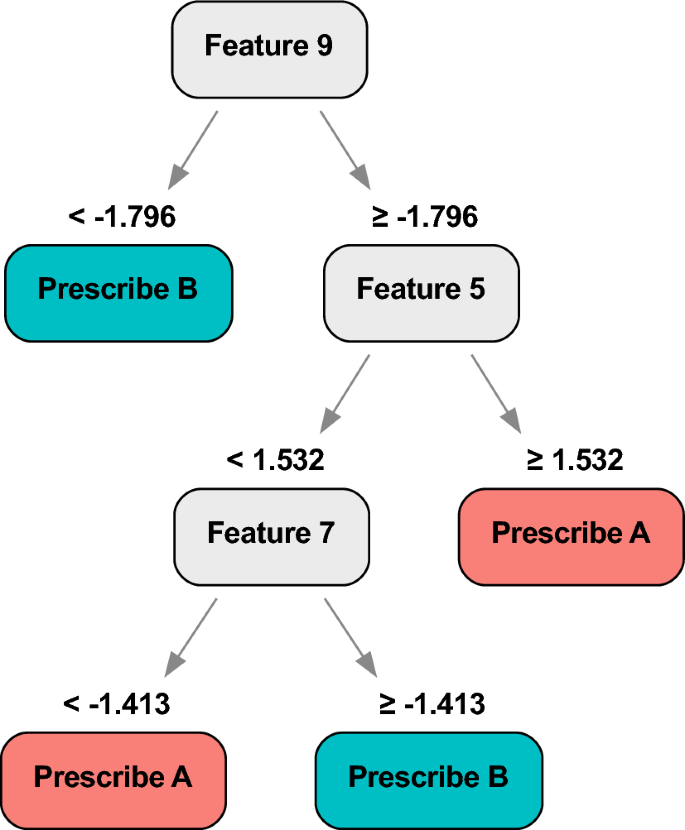
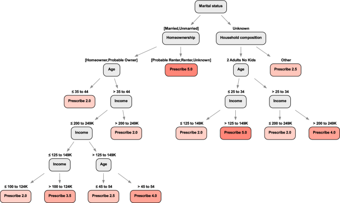
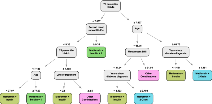
We show an example of the Optimal Policy Tree (continuous dosing) output in Fig. 8 trained with 1,000 data points. We can see that it uses the patient’s recent HbA1c history, age, current line of treatment, years since previous diagnosis, and BMI to prescribe from the variety of treatments. This tree, with 10 leaves, is significantly smaller than the best Optimal Prescriptive Tree, which had 21 leaves, with similar performance. This is strong evidence that separating the counterfactual estimation from the policy learning results in more concise trees that focus solely on the factors that affect treatment assignment. In contrast, the Optimal Prescriptive Trees are larger because the splits in the tree serve two purposes: refining the counterfactual estimation and determining the optimal treatment policy.
In this section, we apply Optimal Policy Trees to develop a new interpretable pricing methodology for exchange-traded financial instruments (e.g. stocks, bonds, etc.). For commercial sensitivity reasons, some details of the study are omitted and the tree we show is illustrative.
The problem we consider is predicting the future price of an asset at some time in the near future (on the order of minutes). The data available for prediction is the transaction history of this and other assets as well as all buy/sell orders on the market and their price points.
There are many approaches to predict future prices from this information. For instance, a common calculation is the mid-price, which is the average price of the highest “buy” (bid price) and lowest “sell” (ask price) orders. Another is the weighted mid-price, which is similar but weights the average by the size of the orders. There are many such pricing formulae that consider various aspects of the historical data (e.g. historical transaction prices, momentum prices, high-liquidity prices, etc.), and these are often highly-complex non-linear formulae that have been hand-designed based on domain expertise. In collaboration with domain experts, we identified nearly 200 such pricing formulae that are regularly used. It is known that different formulae perform well in some market conditions and poorly in others, but this is based loosely on human intuition and not directly understood in a quantitative fashion. Given the work and experience that has gone into carefully crafting these highly non-linear formulae, instead of trying to construct our own pricing formula from scratch, we decided to treat each formula as a distinct treatment option and attempt to learn which formula to apply in different market scenarios to achieve the best price predictions.
We applied Optimal Policy Trees to develop a policy for which pricing methodology is best to use under different market conditions. Mathematically, each observation i consists of market features \(\varvec<\mathbf
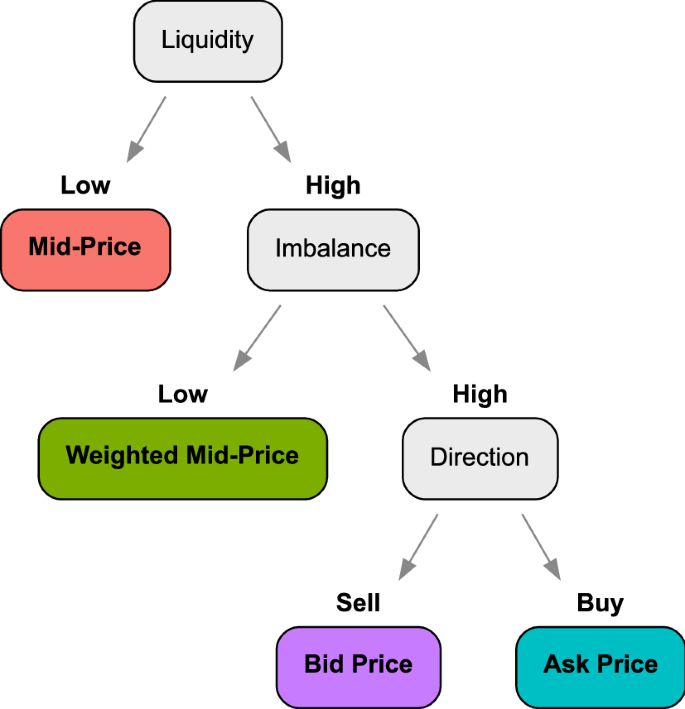
An example of the Optimal Policy Trees learned on the data is shown in Fig. 9. We observe that the tree prescribes the mid-price when liquidity is low: this is consistent with the intuition that in such conditions, most of the market signals are noisy and the best choice is to simply average the bid and ask prices. On the other hand, in high liquidity conditions, the tree then splits on order imbalance, picking the weighted mid-price as the best estimator when the number of orders on the buy and sell sides are similar and the market is balanced. On the other hand, if the sizes of buy and sell orders are highly imbalanced, the tree then splits on the direction of the disparity to either assign the ask price if the bias is towards the “buy” side, or the bid price if the bias is towards the “sell” side, mirroring the fundamental dynamics of supply and demand. Together, the splits of this tree provide a clear and understandable formalization of when each price is best that is aligned with human intuition.
In comprehensive out-of-sample testing, the pricing approaches developed using Optimal Policy Trees consistently outperformed the existing approaches to pricing by up to 2% in terms of accuracy of future price predictions, and the interpretability and transparency of the models allow humans to derive insights and further their own understanding of the problem.
In this paper, we presented an interpretable approach for learning optimal prescription policies, combining the state-of-the-art in counterfactual estimation from the causal inference literature with the power of modern techniques for global decision tree optimization. The resulting Optimal Policy Trees are highly interpretable and scalable, and our experiments showed that they offer best-in-class performance, outperforming similar greedy approaches, and make extremely efficient use of data compared to prescriptive tree methods.
Finally, we showed in a number of real-world applications that this approach results in prescription policies of significantly higher quality when compared to existing approaches.
This framework of learning prescription policies is very general and invites many paths for potential future work. For example, one might consider multi-output scenarios where a prescription could affect several outputs at once. Another avenue could be considering constraints on which treatments can be applied to each observation depending on their features.
The dataset used in Section 4.1 is publicly available. The datasets used in Sections 4.2 and 4.3 are confidential.
The code implementing the experiments is available upon request. The code implementing the Optimal Policy Tree algorithm is available under a free academic license from Interpretable AI LLC.
The work was conducted by the authors while employed by Interpretable AI LLC.